As part of my recent work, I’ve been using a lot of OpenSearch’s vector search. As it’s quite a new topic for me, I thought it would be worth writing up my thoughts and understanding of the tech. Hopefully you find it useful too!
Vector Embeddings
So, an initial point for vector searching (sometime known as semantic searching) is setting up an index which will store your vector embeddings
So what is a vector embedding!? Vector embeddings are essentially co-ordinates in the form of a vector [0.4, -0.87, 0.1263, ...] that map the meaning of a word or chunk of text. (Most unstructured data can also be vectorised, including images! However, I’ve not done much work on semantic searching of images… yet.)
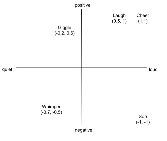
In the diagram above, you can see an example of some words mapped onto a very simple two-dimensional space with two parameters, loudness (x-axis) and positivity (y-axis).
In this case the words above would have vectors of:
- Cheer [1, 1]
- Laugh [0.5, 1]
- Giggle [-0.2, 0.6]
- Whimper [-0.7, -0.5]
- Sob [-1, -1]
From the above, we can see easily which words have a similar meaning within our parameters; for example, both a laugh and a cheer are both very positive and quite loud and so are close in semantic meaning (and are physically close on our map).
Of course, realistically, the embeddings generated by LLM models have an incredibly higher number of dimensions (typically 384, 768, 1024, or even higher depending upon the model). This allows them to store much more semantic information that my two dimensional diagram above!
These systems capture much more context, including synonyms, themes, etc. For example, “dog” and “chihuahua” would match relatively closely on that multi-dimensional vector.
How does this become a search?
So, OpenSearch measures the mathematical distance (in meaning) between a query that a user has entered, and vectors that are stored in our indexed database. When a user enters a query, that query is run through the exact same embedding model that was used to generate our indexed database. The user’s query vector is then used to find a similar match (or matches).
There are a few main methods for calculating this distance “Cosine similarity”, “Euclidean distance” and “Dot product”.
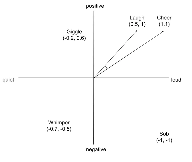
Cosine Similarity
This method measures the angle between vectors, using the origin [0, 0, 0, …, 0] as the starting point. The benefit of using cosine similarity is that it has a greater focus on thematic meaning when matching two vectors. It does not matter if one vector represents a small paragraph, whilst another represents 10s of pages of a document.
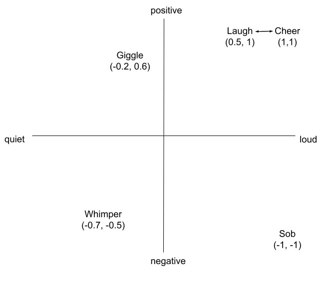
Euclidean distance
Meanwhile, Euclidean distance measures the distance between the endpoints of two vectors.
This tends to be better for fixed length data, or image vectors where the absolute magnitude of the vector matters more.
Dot product
There is another matching method called Dot product which combines both the direction (like with cosine) and magnitude (like with euclidean). This results in a match that is influenced by both the angle and magnitude. For example, a longer vector can still score well even if the angle is slightly worse.
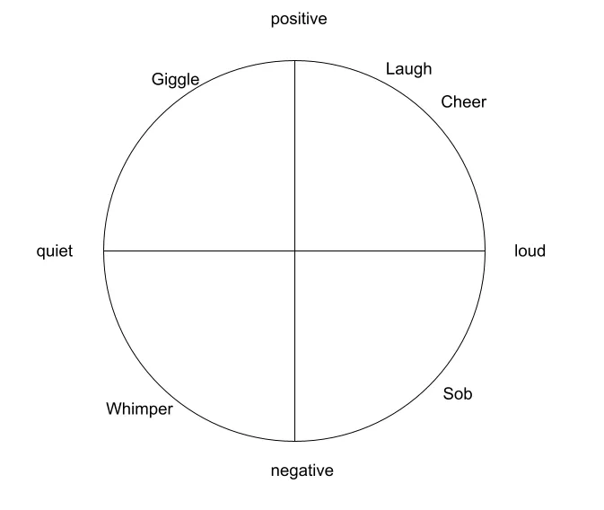
However, another option is to first normalise the vectors. This means making all vectors have the same magnitude (i.e. distance from (0, 0, 0, …, 0)).
In our two-dimensional example, if we normalise the vectors to have a magnitude of 1, we’d expect all vectors to end on a circle of radius 1 from (0, 0). The same would be true on a three-dimensional map with a consistent radius of 1 (think a globe), and continuing up into many dimensional hyper-spheres.
At the point that things are normalised, the results from a dot product match should be the same as a cosine match. However, the speed of the match should be quicker because the system no longer has to consider the length of the vectors on the fly.
Scaling search (HNSW)
So all of my examples so far have used the initial simple two-dimensional map. However, when there may be hundreds of thousands, to millions of records, mapped against up to 1,024 dimensions, calculating the distance between one user’s query and millions of documents becomes computationally prohibitive. (It is an $O(N)$ complexity operation).
As such, OpenSearch uses something called Hierarchical Navigable Small World (HNSW) graphs. This brings the operation down to $O(\log N)$, meaning that this search is much more scalable.
The way this works is that rather than doing a full vector comparison against the whole data-set, the vector is compared against a multi-layer graph.
Each layer is a network of real vectors from your dataset. The higher the layer, the fewer vectors there are, but the longer the “jumps” between them. The bottom layer contains every vector with dense, short-range connections.
A common way of visualising these levels is as a transport network.
- The highest level is the motorway system, getting you into a general area with fewer stopping points.
- The next level is the local streets within the city you’ve arrived at. These are more numerous and get you a lot closer to your destination.
- Finally, you hit the local street for your destination and you are looking at individual houses for matches.
But I need to be able to make exact match searches! 😭
Realistically, when doing a search, end users still expect to be able to make exact matches alongside these newer semantic searches. So how do we do this!?
Thankfully, OpenSearch has the ability to run hybrid searches, which combines the results of an exact keyword search with the results of a semantic search.
It achieves this by running an exact keyword search and a semantic search in parallel, and then combining the results of both of these by using Reciprocal Rank Fusion (RRF). This is required due to the ranking systems of these two search systems being different.
RRF combines these ranks and favours results that rank highly on both exact match and semantic searches. This prevents one result that ranks very highly on one search from dominating the results if it’s a bad match within the other system.
Comments
Loading comments...